Originally published as a cookbook on docs.telemetry.mozilla.org to instruct data users within Mozilla how to take advantage of the usage history stored in our BigQuery tables.
Monthly active users (MAU) is a windowed metric that requires joining data
per client across 28 days. Calculating this from individual pings or daily
aggregations can be computationally expensive, which motivated creation of the
clients_last_seen dataset
for desktop Firefox and similar datasets for other applications.
A powerful feature of the clients_last_seen methodology is that it doesn’t
record specific metrics like MAU and WAU directly, but rather each row stores
a history of the discrete days on which a client was active in the past 28 days.
We could calculate active users in a 10 day or 25 day window just as efficiently
as a 7 day (WAU) or 28 day (MAU) window. But we can also define completely new
metrics based on these usage histories, such as various retention definitions.
The usage history is encoded as a “bit pattern” where the physical type of the field is a BigQuery INT64, but logically the integer represents an array of bits, with each 1 indicating a day where the given clients was active and each 0 indicating a day where the client was inactive. This article discusses the details of how we represent usage in bit patterns, how to extract standard usage and retention metrics, and how to build new metrics from them.
Calculating DAU, WAU, and MAU
The simplest application of usage bit patterns is for calculating metrics in backward-looking windows. This is what we do for our canonical usage measures DAU, WAU, and MAU.
To decide whether a given client should count towards DAU, WAU, and MAU, we need to know how recently that client was active. If the client was seen in the past 28 days, they count toward MAU. If they were active in the past 7 days, the count toward WAU. And only if they were active today do they count toward DAU.
The user-facing clients_last_seen views present fields like days_since_seen
that extract this information for us from the underlying days_seen_bits field,
allowing us to easily express DAU, WAU, and MAU aggregates like:
SELECT
  submission_date,
  COUNTIF(days_since_seen < 28) AS mau,
  COUNTIF(days_since_seen <  7) AS wau,
  COUNTIF(days_since_seen <  1) AS dau
FROM
  telemetry.clients_last_seen
WHERE
  submission_date = '2020-01-28'
GROUP BY
  submission_date
ORDER BY
  submission_date
Under the hood, days_since_seen is calculated using the bits28_days_since_seen
UDF which is explained in more detail later in this article.
Note that the desktop clients_last_seen table also has additional bit pattern
fields corresponding to other usage criteria,
so other variants on MAU can be calculated like:
SELECT
  submission_date,
  COUNTIF(days_since_visited_5_uri < 28) AS visited_5_uri_mau,
  COUNTIF(days_since_opened_dev_tools < 28) AS opened_dev_tools_mau
FROM
  telemetry.clients_last_seen
WHERE
  submission_date = '2020-01-28'
GROUP BY
  submission_date
ORDER BY
  submission_date
Also note that non-desktop products also have derived tables following the
clients_last_seen methodology. Per-product MAU could be calculated as:
SELECT
  submission_date,
  app_name,
  COUNTIF(days_since_seen < 28) AS mau,
  COUNTIF(days_since_seen <  7) AS wau,
  COUNTIF(days_since_seen <  1) AS dau
FROM
  telemetry.nondesktop_clients_last_seen
WHERE
  submission_date = '2020-01-28'
GROUP BY
  submission_date, app_name
ORDER BY
  submission_date, app_name
Calculating retention
For retention calculations, we use forward-looking windows. This means that when we report a retention value for 2020-01-01, we’re talking about what portion of clients active on 2020-01-01 are still active some number of days later.
In particular, let’s consider the “1-Week Retention” measure shown in GUD which considers a window of 14 days. For each client active in “week 0” (days 0 through 6), we determine retention by checking if they were also active in “week 1” (days 7 through 13).
We provide a UDF called bits28_retention that returns a rich STRUCT
type representing activity in various windows, with all the date and bit
offsets handled for you. You pass in a bit pattern and the corresponding submission_date,
and it returns fields like:
day_13.metric_dateday_13.active_in_week_0day_13.active_in_week_1
Calculating GUD’s retention aggregates and some other variants looks like:
-- The struct returned by bits28_retention is nested.
-- The first level of nesting defines the beginning of our window;
-- in our case, we want day_13 to get retention in a 2-week window.
-- This base query uses day_13.* to make all the day_13 fields available:
--   - metric_date
--   - active_in_week_0
--   - active_in_week_1
--   - ...
--
WITH base AS (
  SELECT
    *,
    udf.bits28_retention(
      days_seen_bits, submission_date
      ).day_13.*,
    udf.bits28_retention(
      days_created_profile_bits, submission_date
      ).day_13.active_on_metric_date AS is_new_profile
  FROM
    telemetry.clients_last_seen )

SELECT
  metric_date, -- 2020-01-15 (13 days earlier than submission_date)

  -- 1-Week Retention matching GUD.
  SAFE_DIVIDE(
    COUNTIF(active_in_week_1),
    COUNTIF(active_in_week_0)
  ) AS retention_1_week,

  -- 1-Week New Profile Retention matching GUD.
  SAFE_DIVIDE(
    COUNTIF(is_new_profile AND active_in_week_1),
    COUNTIF(is_new_profile)
  ) AS retention_1_week_new_profile,

  -- NOT AN OFFICIAL METRIC
  -- A more restrictive 1-Week Retention definition that considers only clients
  -- active on day 0 rather than clients active on any day in week 0.
  SAFE_DIVIDE(
    COUNTIF(active_in_week_1),
    COUNTIF(active_on_metric_date)
  ) AS retention_1_week_active_on_day_0,

  -- NOT AN OFFICIAL METRIC
  -- A more restrictive 0-and-1-Week Retention definition where again the denominator
  -- is restricted to clients active on day 0 and the client must be active both in
  -- week 0 after the metric date and in week 1.
  SAFE_DIVIDE(
    COUNTIF(active_in_week_0_after_metric_date AND active_in_week_1),
    COUNTIF(active_on_metric_date)
  ) AS retention_0_and_1_week_active_on_day_0,

FROM
  base
WHERE
  submission_date = '2020-01-28'
GROUP BY
  metric_date
Under the hood, bits28_retention is using a series of calls to the lower-level
bits28_range function, which is explained later in this article.
bits28_range is very powerful and can be used to construct novel metrics,
but it also introduces many opportunities for off-by-one errors and passing parameters
in incorrect order, so please fully read through this documentation before
attempting to use the lower-level functions.
Understanding bit patterns
If you look at the days_seen_bits field in telemetry.clients_last_seen,
you’ll see seemingly random whole numbers, some as large as nine digits.
How should we interpret these?
For very small numbers, it may be possible to interpret the value by eye.
A value of 1 means the client was active on submission_date only
and wasn’t seen in any of the 27 days previous. A value of 2 means
the client was seen 1 day ago, but not on submission_date. A value of 3
means that the client was seen on submission_date and the day previous.
It’s much easier to reason about these bit patterns, however, when we view them as strings of ones and zeros. We’ve provided a UDF to convert these values to “bit strings”:
SELECT
  [ udf.bits28_to_string(1),
    udf.bits28_to_string(2),
    udf.bits28_to_string(3) ]

>>> ['0000000000000000000000000001',
     '0000000000000000000000000010',
     '0000000000000000000000000011']
A value of 3 is equal to 2^1 + 2^0 and indeed we see that reading from
right to left in the string of bits, the “lowest” to bits are set (1) while
the rest of the bits are unset (0).
Let’s consider a larger value 8256. In terms of powers of two, this is equal
to 2^13 + 2^6 and its string representation should have two 1 values.
If we label the rightmost bit as “offset 0”, we would expect the set
bits to be at offsets -13 and -6:
SELECT udf.bits28_to_string(8256)

>>> '0000000000000010000001000000'
We also provide the inverse of this function to take a string representation of a bit pattern and return the associated integer:
SELECT udf.bits28_from_string('0000000000000010000001000000')

>>> 8256
Note that the leading zeros are optional for this function:
SELECT udf.bits28_from_string('10000001000000')

>>> 8256
Finally, we can translate this into an array of concrete dates by passing a value for the date that corresponds to the rightmost bit:
SELECT udf.bits28_to_dates(8256, '2020-01-28')

>>> ['2020-01-15', '2020-01-22']
Why 28 bits instead of 64?
BigQuery has only one integer type (INT64) which is composed of 64 bits,
so we could technically store 64 days of history per bit pattern. Limiting
to 28 bits is a practical concern related to storage costs and reprocessing concerns.
Consider a client that is only active on a single day and then never shows up again.
A client that becomes inactive will eventually fall outside the 28-day usage
window and will thus not have a row in following days of clients_last_seen
and we no longer duplicate that client’s data for those days.
Also, tables following the clients_last_seen methodology have to be populated
incrementally. For each new day of data, we have to reference the previous
day’s rows in clients_last_seen, take the trailing 27 bits of each pattern
and appending a 0 or 1 to represent whether the client was active in the new
day.
Now, suppose we find that there was a processing error 10 days ago that affected
a table upstream of clients_last_seen. If we fix that error, we now have to
recompute each day of clients_last_seen from 10 days ago all the way to the
present.
We chose to encode only 28 days of history in these bit patterns as a compromise that gives just enough history to calculate MAU on a rolling basis but otherwise limits the amount of data that needs to be reprocessed to recover from errors.
Forward-looking windows and backward-looking windows
Bit patterns can be used to calculate a variety of windowed metrics, but there are a number of ways we can choose to interpret a bit pattern and define windows within it. In particular, we can choose to read a bit pattern from right to left, looking backwards from the most recent day. Or we can choose to read a bit pattern from left to right, looking forwards from some chosen reference point.
MAU and WAU use backward-looking windows where the value for 2020-01-28
depends on activity from 2020-01-01 to 2020-01-28. You can calculate DAU,
WAU, and MAU for 2020-01-28 as soon data for that target date has been
processed. In other words, the metric date for usage metrics corresponds
directly to the submission_date in clients_last_seen.
Retention metrics, however, use forward-looking windows where the value for
2020-01-28 depends on activity happening on and after that date.
Be prepared for this to twist your mind a bit. What we call “1-Week Retention”
depends on activity in a 2-week window. If we want to calculate a 1-week
retention value for 2020-01-01, we need to consider activity from 2020-01-01
through 2020-01-14, so we cannot know the retention value for a given day
until we’ve fully processed data 13 days later. In other words, the metric date
for 1-week retention is always 13 days earlier than the submission_date
on which it can be calculated.
Using forward-looking windows initially seems awkward, but it turns out to be necessary for consistency in how we define various retention metrics. Consider if we wanted to compare 1-week, 2-week, and 3-week retention metrics on a single plot. If we use forward-looking windows, then the point labeled 2020-01-01 describes the same set of users for all three metrics and how their activity differs over time. If we use backwards-looking windows, then each of these three metrics is considering a separate population of users. We’ll discuss this in more detail later.
Usage: Backward-looking windows
The simplest application of usage bit patterns is for calculating metrics in backward-looking windows. This is what we do for our canonical usage measures DAU, WAU, and MAU.
Let’s imagine a single row from clients_last_seen with submission_date = 2020-01-28.
The days_seen_bits field records usage for a single client over a period of 28 days
ending on the given submission_date. We will call this metric date “day 0”
(2020-01-28 in this case) and count backwards to “day -27” (2020-01-01).
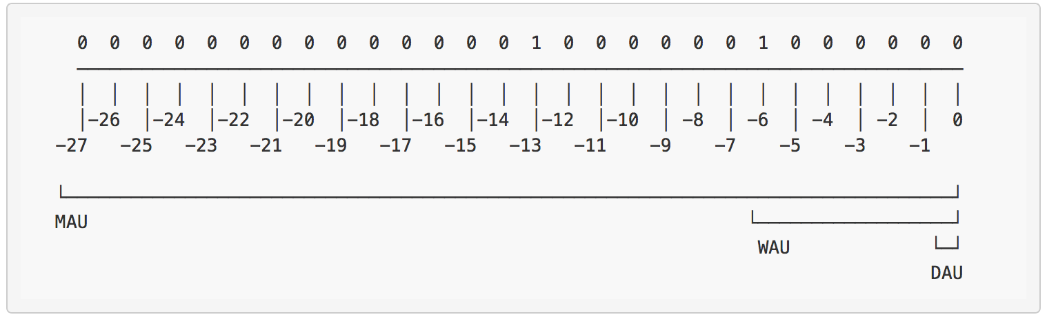
Let’s suppose this client was only active on two days in the past month:
2020-01-22 (day -6) and 2020-01-15 (day -13). That client’s days_seen_bits
value would show up as 8256, which as we saw in the previous section can
be represented as bit string '0000000000000010000001000000'.
Let’s dive more deeply into that bit string representation:
    0  0  0  0  0  0  0  0  0  0  0  0  0  0  1  0  0  0  0  0  0  1  0  0  0  0  0  0
    ──────────────────────────────────────────────────────────────────────────────────
    │  │  │  │  │  │  │  │  │  │  │  │  │  │  │  │  │  │  │  │  │  │  │  │  │  │  │  │
    │-26  │-24  │-22  │-20  │-18  │-16  │-14  │-12  │-10  │ -8  │ -6  │ -4  │ -2  │  0
  -27   -25   -23   -21   -19   -17   -15   -13   -11    -9    -7    -5    -3    -1

  └──────────────────────────────────────────────────────────────────────────────────┘
  MAU                                                             └──────────────────┘
                                                                   WAU             └─┘
                                                                                   DAU
In this picture, we’ve annotated the windows for DAU (day 0 only), WAU (days 0 through -6) and MAU (days 0 through -27). This particular client won’t count toward DAU for 2020-01-28, but the client does count towards both WAU and MAU.
Note that for each of these usage metrics, the number of active days does not matter but only the recency of the latest active day. We provide a special function to tell us how many days have elapsed since the most recent activity encoded in a bit pattern:
SELECT udf.bits28_days_since_seen(udf.bits28_from_string('10000001000000'))

>>> 6
Indeed, this is so commonly used that we build this function into user-facing
views, so that instead of referencing days_seen_bits with a UDF, you can
instead reference a field called days_since_seen. Counting MAU, WAU, and
DAU generally looks like:
SELECT
  COUNTIF(days_since_seen < 28) AS mau,
  COUNTIF(days_since_seen <  7) AS wau,
  COUNTIF(days_since_seen <  1) AS dau
FROM
  telemetry.clients_last_seen
How windows shift from day to day
Note that this particular client is about to fall outside the WAU window.
If the client doesn’t send a main ping on 2020-01-29, the new days_seen_bits
pattern for this client will look like:
    0  0  0  0  0  0  0  0  0  0  0  0  0  1  0  0  0  0  0  0  1  0  0  0  0  0  0  0
    ──────────────────────────────────────────────────────────────────────────────────
    │  │  │  │  │  │  │  │  │  │  │  │  │  │  │  │  │  │  │  │  │  │  │  │  │  │  │  │
    │-26  │-24  │-22  │-20  │-18  │-16  │-14  │-12  │-10  │ -8  │ -6  │ -4  │ -2  │  0
  -27   -25   -23   -21   -19   -17   -15   -13   -11    -9    -7    -5    -3    -1

  └──────────────────────────────────────────────────────────────────────────────────┘
  MAU                                                             └──────────────────┘
                                                                   WAU             └─┘
                                                                                   DAU
The entire pattern has simply shifted one offset to the left, with the leading zero
falling off (since it’s now outside the 28-day range) and a trailing zero added
on the right (this would be a 1 instead if the user had been active on 2020-01-29).
The days_since_seen value is now 7, which is outside the WAU window:
SELECT udf.bits28_days_since_seen(udf.bits28_from_string('100000010000000'))

>>> 7
Retention: Forward-looking windows
For retention calculations, we use forward-looking windows. This means that when we report a retention value for 2020-01-01, we’re talking about what portion of clients active on 2020-01-01 are still active some number of days later.
When we were talking about backward-looking windows, our metric date or “day 0” was always the most recent day, corresponding to the rightmost bit. When we define forward-looking windows, however, we always choose a metric date some time in the past. How we number the individual bits depends on what metric date we choose.
For example, in GUD, we show a “1-Week Retention” which considers a window of 14 days. For each client active in “week 0” (days 0 through 6), we determine retention by checking if they were also active in “week 1” (days 7 through 13).
To make “1-Week Retention” more concrete,
let’s consider the same client as before, grabbing the days_seen_bits value from
clients_last_seen with submission_date = 2020-01-28. We count back 13 bits in
the array to define our new “day 0” which corresponds to 2020-01-15:
    0  0  0  0  0  0  0  0  0  0  0  0  0  0  1  0  0  0  0  0  0  1  0  0  0  0  0  0
    ──────────────────────────────────────────────────────────────────────────────────
                                              │  │  │  │  │  │  │  │  │  │  │  │  │  │
                                              │  1  │  3  │  5  │  7  │  9  │ 11  │ 13
                                              0     2     4     6     8    10    12
                                            └────────────────────┘
                                                    Week 0       └───────────────────┘
                                                                        Week 1
This client has a bit set in both week 0 and in week 1, so logically this client can be considered retained; they should be counted in both the denominator and in the numerator for the “1-Week Retention” value on 2020-01-15.
Also note there is some nuance in retention metrics as to what counts as “week 0” because sometimes we want to measure a user as active in week 0 excluding the metric date (“day 0”) itself. The client shown above would not count as “active in week 0 after metric date”:
    0  0  0  0  0  0  0  0  0  0  0  0  0  0  1  0  0  0  0  0  0  1  0  0  0  0  0  0
    ──────────────────────────────────────────────────────────────────────────────────
                                              │  │  │  │  │  │  │  │  │  │  │  │  │  │
                                              │  1  │  3  │  5  │  7  │  9  │ 11  │ 13
                                              0     2     4     6     8    10    12
                             Metric Date    └──┘
                Week 0 After Metric Date       └─────────────────┘
                                  Week 0    └────────────────────┘
But how can we extract this usage per week information in a query?
Extracting the bits for a specific week can be achieved via UDF:
SELECT
  -- Signature is bits28_range(offset_to_day_0, start_bit, number_of_bits)
  udf.bits28_range(days_seen_bits, -13 + 0, 7) AS week_0_bits,
  udf.bits28_range(days_seen_bits, -13 + 7, 7) AS week_1_bits
FROM
  telemetry.clients_last_seen
And then we can turn those bits into a boolean indicating whether the client was active or not as:
SELECT
  BIT_COUNT(udf.bits28_range(days_seen_bits, -13 + 0, 7)) > 0 AS active_in_week_0
  BIT_COUNT(udf.bits28_range(days_seen_bits, -13 + 7, 7)) > 0 AS active_in_week_1
FROM
  telemetry.clients_last_seen
This pattern of checking whether any bit is set within a given range is common
enough that we provide short-hand for it in bits28_active_in_range.
The above query can be made a bit cleaner as:
SELECT
  udf.bits28_active_in_range(days_seen_bits, -13 + 0, 7) AS active_in_week_0
  udf.bits28_active_in_range(days_seen_bits, -13 + 7, 7) AS active_in_week_1
FROM
  telemetry.clients_last_seen
In terms of the higher-level bits28_retention function discussed earlier,
here’s how this client looks:
SELECT
  submission_date,
  udf.bits28_retention(days_seen_bits, submission_date).day_13.*
FROM
  telemetry.clients_last_seen

/*
                   submission_date = 2020-01-28
                       metric_date = 2020-01-15
                   active_on_day_0 = true
                  active_in_week_0 = true
active_in_week_0_after_metric_date = false
                  active_in_week_1 = true
*/
N-day Retention
Not an official metric. This section is intended solely as an example of advanced usage.
As an example of a novel metric that can be defined using the low-level
bit pattern UDFs, let’s define n-day retention as the fraction of clients active on a given day
who are also active within the next n days. For example, 3-day retention would
have a denominator of all clients active on day 0 and a numerator of all clients
active on day 0 who were also active on days 1 or 2.
To calculate n-day retention, we need to use the lower-level bits28_range
function:
DECLARE n INT64;
SET n = 3;

WITH base AS (
  SELECT
    *,
    udf.bits28_active_in_range(days_seen_bits, -n + 1, 1) AS seen_on_day_0,
    udf.bits28_active_in_range(days_seen_bits, -n + 2, n - 1) AS seen_after_day_0
  FROM
    telemetry.clients_last_seen )
SELECT
  DATE_SUB(submission_date, INTERVAL n DAY) AS metric_date,

  -- NOT AN OFFICIAL METRIC
  SAFE_DIVIDE(
    COUNTIF(seen_on_day_0 AND seen_after_day_0),
    COUNTIF(seen_on_day_0)
  ) AS retention_n_day
FROM
  base
WHERE
  submission_date = '2020-01-28'
GROUP BY
  metric_date
Retention using activity date
Not an official metric. This section is intended solely as an example of advanced usage.
GUD’s canonical retention definitions are all based on ping submission dates rather
than logical activity dates taken from client-provided timestamps, but there is
interest in using client timestamps particularly for n-day retention calculations
for mobile products.
Let’s consider Firefox Preview which sends telemetry via Glean. The
org_mozilla_fenix.baseline_clients_last_seen table includes two bit patterns
that encode client timestamps: days_seen_session_start_bits and
days_seen_session_end_bits. This table is still populated once per day based
on pings received over the previous day, but some of those pings will reflect
sessions that started on previous days. This introduces some new complexity
into retention calculations because we’ll always be underestimating client
counts if we have our retention window end on submission_date.
When using activity date, it may be desirable to build in a few days of buffer
to ensure we are considering late-arriving pings. For example, if we wanted
to calculate 3-day retention but allow 2 days of cushion for late-arriving
pings, we would need to use an offset of 5 days from submission_date:
DECLARE n, cushion_days, offset_to_day_0 INT64;
SET n = 3;
SET cushion_days = 2;
SET offset_to_day_0 = 1 - n - cushion_days;

WITH base AS (
  SELECT
    *,
    udf.bits28_active_in_range(days_seen_session_start_bits, offset_to_day_0, 1) AS seen_on_day_0,
    udf.bits28_active_in_range(days_seen_session_start_bits, offset_to_day_0 + 1, n - 1) AS seen_after_day_0
  FROM
    org_mozilla_fenix.baseline_clients_last_seen )
SELECT
  DATE_SUB(submission_date, INTERVAL offset_to_day_0 DAY) AS metric_date,

  -- NOT AN OFFICIAL METRIC
  SAFE_DIVIDE(
    COUNTIF(seen_on_day_0 AND seen_after_day_0),
    COUNTIF(seen_on_day_0)
  ) AS retention_n_day
FROM
  base
WHERE
  submission_date = '2020-01-28'
GROUP BY
  metric_date
UDF Reference
See implementations in the bigquery-etl repository.
bits28_to_string
Convert an INT64 field into a 28 character string representing the individual bits.
bits28_to_string(bits INT64)

SELECT udf.bits28_to_string(18)
>> 0000000000000000000000010010
bits28_from_string
Convert a string representing individual bits into an INT64.
bits28_from_string(bits STRING)

SELECT udf.bits28_from_string('10010')
>> 18
bits28_to_dates
Convert a bit pattern into an array of the dates is represents.
bits28_to_dates(bits INT64, end_date DATE)

SELECT udf.bits28_to_dates(18, '2020-01-28')
>> ['2020-01-24', '2020-01-27']
bits28_days_since_seen
Return the position of the rightmost set bit in an INT64 bit pattern.
bits28_days_since_seen(bits INT64)

SELECT bits28_days_since_seen(18)
>> 1
bits28_range
Return an INT64 representing a range of bits from a source bit pattern.
The start_offset must be zero or a negative number indicating an offset from
the rightmost bit in the pattern.
n_bits is the number of bits to consider, counting right from the bit at start_offset.
bits28_range(bits INT64, offset INT64, n_bits INT64)

SELECT udf.bits28_to_string(udf.bits28_range(18, 5, 6))
>> '010010'
SELECT udf.bits28_to_string(udf.bits28_range(18, 5, 2))
>> '01'
SELECT udf.bits28_to_string(udf.bits28_range(18, 5 - 2, 4))
>> '0010'
bits28_active_in_range
Return a boolean indicating if any bits are set in the specified range of a bit pattern.
The start_offset must be zero or a negative number indicating an offset from
the rightmost bit in the pattern.
n_bits is the number of bits to consider, counting right from the bit at start_offset.
bits28_active_in_range(bits INT64, offset INT64, n_bits INT64)
bits28_retention
Return a nested struct providing numerator and denominator fields for the standard 1-Week, 2-Week, and 3-Week retention definitions.
bits28_retention(bits INT64, submission_date DATE)